GEOTECHNICS AND STATICS OF DRYSTONE WALLS

Technical and calculation supplements to the book
Dry Stone Walls, Basics, Construction, Significance
by Stiftung Umwelt-Einsatz Schweiz

by Theodor Schmidt

The following articles are supplements to the sections "Soil and the Building Ground" and "Dimensioning and Statics" in pages 202 to 237 of the book. They can also be used without the book, but a knowledge of basic walling types and concepts (from page 180 onwards) is helpful. In order to find your way between the book and these supplements, some pages of the book have been inserted here as images - Click them to enlarge.

Much of the following geotechnical information is basic, such as found in many books or lecture notes, however the earth pressure drawing near the end of this document is probably a new type of representation. Similarly, the article on drystone statics commencing with Part I describes known basics, but then in Part II presents some relatively novel equations, a graphical paper-and-pencil representation of these, and a spreadsheet for solving them easily with a computer.

Natural Environment und Context

Pages from the book

198-199

Topography und Terrain

Pages from the book

200-201

202-203

Soil Basics and Mechanics

The soil associated with drystone walls may have several functions:

• as a supporting foundation:
  All drystone walls are built on ground which must offer a sufficient load-carrying capacity.

• as an embankment:
  When an existing retaining wall is removed, the previously internal soil surface is exposed as a bank. Also when building a new retaining wall on an existing slope, a temporary bank may result from the initial excavation and may need to be supported. This also applies when building up new terraace, except when this is done at the same time, or after, constructing the wall when the support is present.
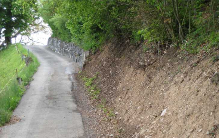
  How steep or high a bank can physically be, is an interesting problem which is described later. How steep and high an embankment can legally be is a question of safety and the corresponding regulations. The following figure summarizes these.
  
  

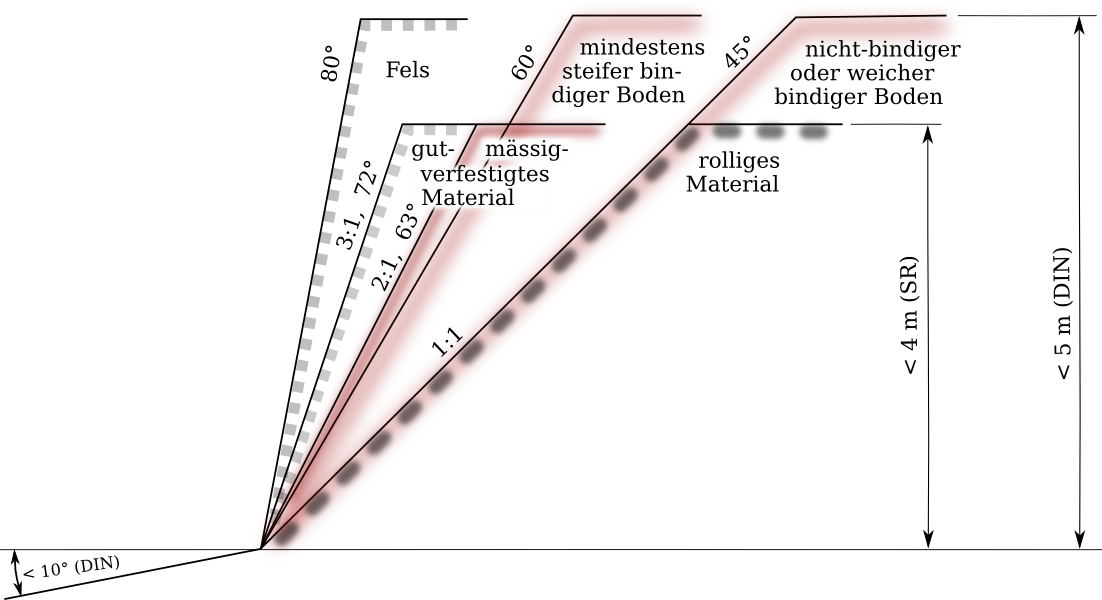
Permissible slope angles and heights without safety approval according to Art. 56 of the Swiss Regulation SR 832.311.141 and/or the German standard DIN 4124 (10.02), if not loaded by heavy loads (SR), not freshly backfilled (DIN), and not impaired by water influx (both).

• as backfill:
  Unless the retaining wall is built right up to an existing, stable embankment without a gap, there remains between them a volume which must be backfilled with earth or stony material. This unconsolidated backfill leads to lateral earth pressure on the wall and conveys additional pressure from extra surface loads above the wall. Towards the end of this chapter, the calculation of lateral earth pressure is described.

• as building material:
  In some cases drystone walls themselves can be made of soil:
  - as a Clawdd with an extensive earthy backfill (see Clawdd Construction http://www.dswales.org.uk/Publications.html)
  - as a wall made of rammed earth or sun-dried clay bricks
  - as the filling of gabions or sand bags
  These applications are not drystone walls in a strict sense, but belong to the family of sustainable buildings made of stony materials.

In order to assess the suitability of soils for these tasks and to design the necessary structures, their properties must be known. They are described below. First, however, what the soils are actually made of and what they are called must be discussed.

Composition of soils

Soils consist of materials from the crust of the earth and from living things. The rocks of the earth's crust contain silicon as the most common element and are therefore called silicates. After silicon the next most common element is oxygen; both together are contained in quartz, which is chemically silicon dioxide (SiO₂). Some special organisms, diatoms, also make SiO₂, which is deposited in the form of diatomaceous earth or kieselguhr. These are very small, amorphous (unstructured) particles, in contrast to the silicates, which form crystals.

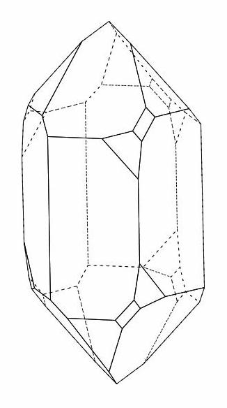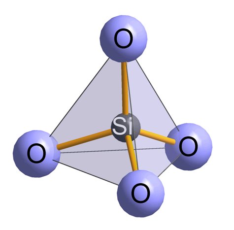
The structure of quartz is important: In the smallest unit (picture on the left) a silicon atom is bonded to four oxygen atoms in a tetrahedron. These units can then bond together in a variety of ways to form bands, layers, or crystals and share the oxygen atoms, so that there are two oxygen atoms for each silicon atom. Depending on the geometry of the bonding, even with 100% SiO₂ various crystal forms and face angles are formed. The picture on the right shows a right-handed quartz crystal.

Most living organisms contain carbon (C), as the most common element after hydrogen and oxygen which occur in water (H₂O). Chemical compounds with carbon are called organic and many solid deposits consist of former organic compounds. Many organisms, however, can collect a large amount of calcium in their skeletons, for example corals and shells. The most common compound is calcium carbonate (CaCO₃) and the remains of such marine animals form coral reefs, sands and sediments which become limestone, marble and chalk after a geological process. These rocks, together with the silicates, play a major role in drystone building, whether as building stones or as components of the ground. Limestone is slightly soluble in water, so that it can be washed out in long periods of time to form cavities and caves, but may also be re-deposited, for example as stalagmites.

In the ground there are also plant roots and countless animals, such as worms, insects, fungi, and bacteria. When these die, they become humus, as do the aboveground components of the plants which fall to the ground, and make up a layer, usually a few centimeters thick. Through animal and agricultural activities, the components of humus and other substances such as fertilizers infiltrate the upper soil layer, sometimes referred to as topsoil or mother soil. This is soft and decomposes rapidly, so it is a poor material on which to build. In most soils the humus content, however, quickly decreases away from the surface and can be seen as a change from a dark to a lighter color.

Soils which were able to develop relatively undisturbed over millennia are referred to as virgin, mature, natural, or original soils. Lake https://en.wikipedia.org/wiki/Pedogenesis. They can be described as a stack of several horizontal layers called horizons. Lake https://en.wikipedia.org/wiki/Soil_horizon

Under this surface is the bedrock formed by geological processes. Near the surface this begins to weather due to air, water, temperature fluctuations, and chemical and biological influences. Cracks appear and rocks or stones are formed. Closer to the surface, the stones are smaller and the grain of the aggregate is finer. Additional material is brought by wind and water. The very finest grains (clay) originate by chemical modification. The variously sized grains mix and form a relatively firm, naturally compacted, subsoil with hardly any humus content. On this lies the topsoil, which can contain up to a third of humus. A mature soil stratified in the manner takes thousands of years to form.

The bedrock is pushed upward in many places by the movements of the earth's crust is. Here the mostly solid, sometimes semi-solid rock comes directly to the surface, for example as mountain peaks. These are constantly being eroded and crumble, allowing cliffs and below these scree slopes to form. Water and ice work on the rock to form cliffs and gorges and this produces gravel, sand and finer particles.

Soils can be freshly deposited by water, wind or gravity to form sand dunes, beaches, gravel banks or scree slopes in the mountains, and of course they can be heaped artifically.

Between the grains are pores filled partly with air and partly with water as well as dissolved substances. Fine-grained soils give rise to large surface areas - relative to their mass - to which other substances can cling.

Characterization of soils

Various natural and engineering sciences deal with the complex issues of soils. Thus there are different approaches for characterizing and specifying soils derived from their:

• formation (geology), or origin (geography)

• chemical composition

• biological or agricultural use

• morphology, i.e. shape and size

• appearance or properties

• technical properties or engineering quality

For drystone construction it seems suitable to follow the terminology as most commonly used for engineering purposes. The figure of the particle size distribution shows the classification according to the international scale ISO 14688-1. The measure of grain diameter refers to the average grain diameter or characteristic size of a measurement method such as sieves. See https://en.wikipedia.org/wiki/Grain_size.

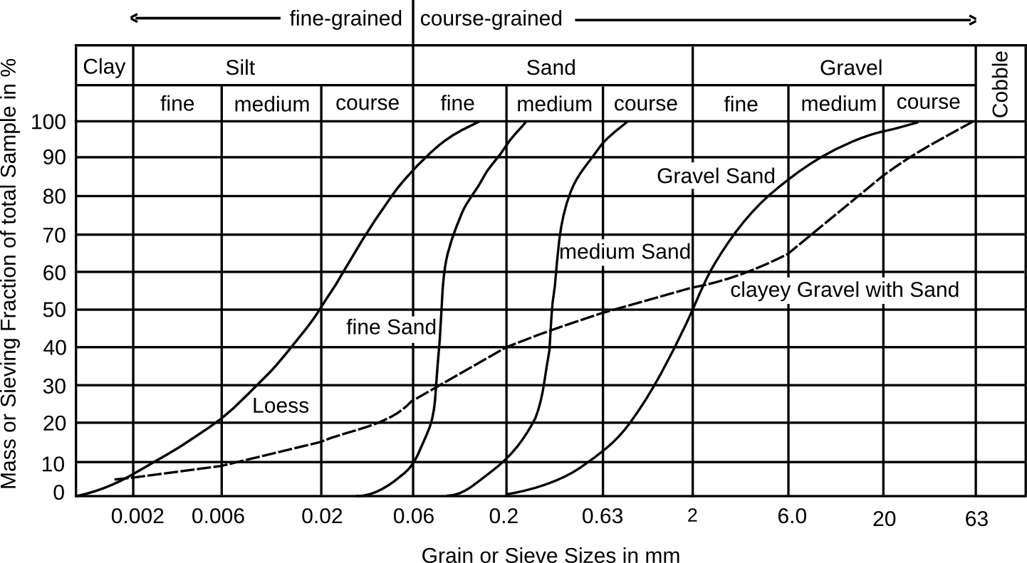
Particle size distribution: In nature, there are no soils with a single grain size; even close-grained materials have a proportion of finer and of coarser grains. The grain sizes of widely graded soils vary over a large range. For example: The material designated 'gravelly sand' contains 15% by weight medium sand, 35% coarse sand, 34% fine gravel, 14% medium gravel and 2% course gravel.

The boundary between fine-grained and coarse-grained is not the same for all the classification schemes. Sometimes it is at 2 mm and the courser grains are called the skeleton of the soil. Or the grain size is further divided into course, medium, fine, very fine, etc.

In the international scale a stone or grain size over 63 millimeters in size is called cobble (Co), over 200 millimeters boulder (Bo), and at over 630 mm large boulder (LBo).

Grain sizes between 2 and 63 mm are called gravel (Gr), between 0.063 and 2 mm Sand (Sa).

Besides the size, the grain shape is important, so there are terms such as rounded, angular, or sharp. Often traditional or commercial names are used, e.g. pea gravel (rounded), or crushed stone (sharp) which is a mechanically crushed material with sharper edges than those that are broken naturally.

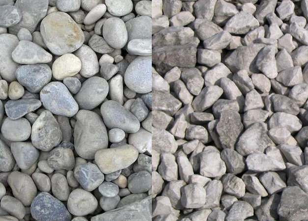
Gravel consists of rounded or angular stones between 2 and 63 mm (left) compared with crushed stone with sharp edges (right).

Particles with sizes finer than 0.063 mm are called silt (Si), and if finer than 0.002 mm clay (Cl). Fine-grained soils are called cohesive because the grains attract each other by an electical binding force called cohesion. The finer the particles, the stronger the cohesion can be.

In nature there are no soils whose grains are all the same size, some are always smaller and some larger. So there is a grain size distribution, which is partly visible but can be determined by sieving. With a stack of sieves with different screen sizes a mixture can be separated. However, this should be done with a standard and defined method, because the amount of material retained in a sieve will also depend somewhat on how long it is shaken. See https://en.wikipedia.org/wiki/Sieve_analysis

Very fine particles are too difficult to sieve; they are separated by forming a suspension in water where the grains separate under the effect of gravity. The process is called sedimentation. Larger grains sink faster to the bottom than finer ones. See http://www.cpsinstruments.eu/pdf/Introduction Differential Sedimentation.pdf

If the mass fractions of a soil are determined, they can be entered in a diagram as a function of the grain size. It is common to use a chart type called sum diagram, as in the figure above showing the grain size distribution. The curves give information of the nature of the soil. With steep curves the majority of particles is within a single grain size designation and the description is clear. For example, as in the case of the curves for "fine sand" and "medium sand". Such mixtures are referred to as "well sorted", "closely" or "poorly graded". With flatter curves over a large range the mixtures are called "poorly sorted" "wide" or "well graded". An example is the curve called "sandy gravel".

Soil classification

Soils are sometimes referred to using their grain sizes, but this only works well with poorly-graded soils. Well-graded soils need additional designations. However, there are different definitions. For example, in the German standard DIN 18196 a soil is called coarse if less than 5% of the mass is silt or clay and more than 40% is at least of gravel-particle size. A soil is considered fine if more than 40% of its mass is fine-grained. In the relevant Swiss standard, however, coarse-grained soils are those with 50% or more of at least sand-grain sizes (> 0.063 mm), and fine-grained soils as those with 50% or more silt or clay grain sizes. In the American Unified Soil Classification System the division is similar, but the sand-silt boundary is at 0.075 mm instead of 0.063 mm and other abreviations are used for the grain sizes, e.g. M for silt. Then there are soils with both a high percentage of fines as well as coarse grains. An example is the curve "clayey gravel with sand" shown in the figure.

Gravel-sand mixtures are also sold under various trade names, depending on their origin, composition or purpose of use. E.g. bank gravel, pea gravel, rock chippings, grit, or frost protection gravel. Often the compositions are defined exactly in diagrams.

Although still belonging to the coarse-grained soils, sands form the transition to the fine-grained soils. Pure sands are usually closely graded and have special features.

Fine particles together with sand form a wide variety of different clay mixtures and subspecies. Since sedimentation in the laboratory and entering in sum charts is rather costly, there are simpler methods of field analysis.

With the method known as the finger probe, a soil sample in the field can be identified by working and feeling with the fingers and observing the resulting deformations. Even for laymen the difference between cohesive and non-cohesive soil is evident. If small rolls can be formed from damp soil between the palms, it is cohesive. Sandy loams feel gritty, silty ones smooth, and clay-rich ones plastic to greasy. The complete process is called called a "pedological mapping procedure". Cf. http://de.wikipedia.org/wiki/Fingerprobe_(Boden) and https://en.wikipedia.org/wiki/Soil_mechanics#Classification_of_silts_and_clays

A common classification method maps loams, i.e. mixtures of clay, silt and sand, into a position on a three-point chart. At a glance the whole loam "family" is visible, including the proportions of clay, silt and sand. Or conversely, if these three mass fractions of a soil are known, it can be classified using the three-point diagram. Up to two dozen subspecies are common, often designated using abbreviations. A capital letter in the first place is the primary designation and one or two lowercase letters the secondary description(s): for example loamy Sand is Sl, clayey loam Lt. For silt or silty U or u is used; loamy silt is thus Ul.

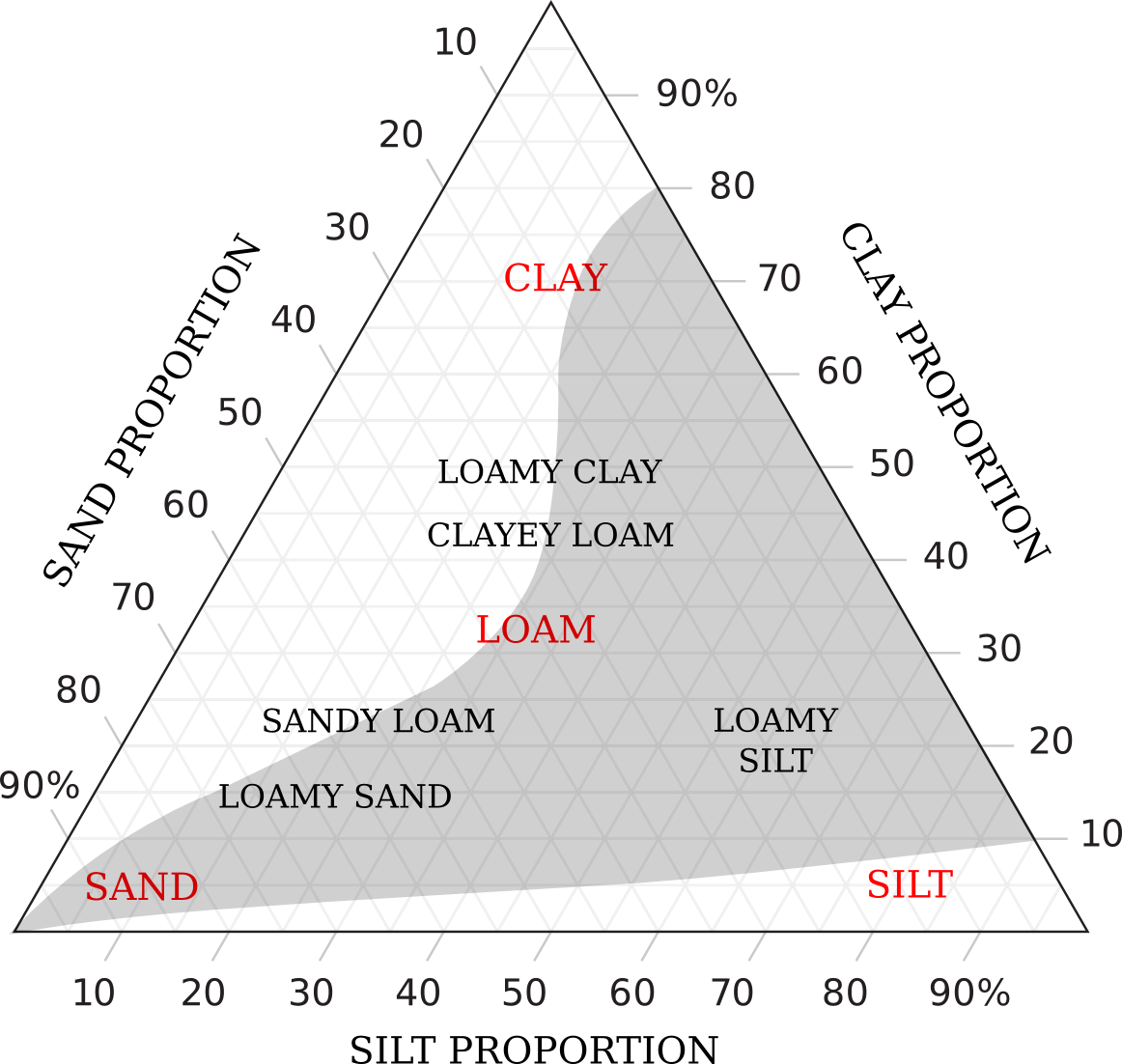
The triangle diagram shows loams depending on the percentage of clay, silt and sand with a few examples. Each point within the triangle describes a sum of three components, which together result in 100%. Examples: loamy Sand (at the "Y"): about 60% sand, 25% silt and 15% clay. A material composed of 60% silt and 20% clay, and 20% sand is loamy silt. The gray coloring shows frequently occurring mixtures (see Hartge 1978). Pure silts, clays, or clay-sands are therefore rare.

Properties of soil

For the construction of free-standing walls, an assessment of the bearing capacity of the soil under the foundation must be known, as well as its settling behaviour. For retaining walls, additionally the earth pressure and influences due to water. Soil is a complex material with many properties or parameters which affect its behavior. In addition to the grain size distribution, the most important are density or specific gravity, void ratio, water content, friction angle and cohesion. Other properties such as the consistency can be calculated from these or measured.

Density and specific gravity

Density, ρ (rho) = mass per unit volume and specific gravity γ (gamma) = weight per unit volume, differ only by the factor of acceleration due to gravity g, because γ = ρ ∙ g. For g one can often use 9.8 or roughly 10 m/s², for a more accurate value see the box.

Acceleration due to gravity: If a mass is released close to the earth's surface, it falls downward with a speed which each second increases by about 10 m/s, that is by 10 m/s per second = 10 m/s². This is often called 1 g, not to be confused with 1 gram. During the accelerated fall the mass is weightless. The acceleration due to gravity however also acts when the mass is at rest on the ground. Between the mass and the ground, the force F_G acts with the value F_G = m ∙ g. This is called the weight.

The acceleration due to gravity g is not constant, but varies according to latitude, altitude, and due to anomalies in the earth's crust. However, the variation is mostly below 1% and as a convention, the standard acceleration of gravity has been globally set to the default value g_n = 9,80665 m/s². For calculating drystone walls it is usually sufficient to use 9.81 or even 10 m/s². However if large quantities of stone are purchased according to weight or mass, it pays to check if these are weighed correctly, and whether the scales used are properly calibrated. Modern electronic scales do not weigh masses as the formerly used balances, but rather measure the force of weight directly, as do spring scales. However the measurement is usually indicated in units of mass, not weight. Such scales therefore give different reading if transported to a place with a different acceleration of gravity. It must then be recalibrated for the relevant gravity zone, otherwise it displays incorrectly. In Switzerland, for very accurate measurements even four gravity zones have been defined, which differ up to 0.5 permille. Otherwise, the average value of g_r = 9,80450 m/s² is valid for Switzerland.(see http://www.metas.ch/metasweb/fachbereiche/waagen/gravitationszonen and http://www.metas.ch/w221.1d (PDF)) With the Online calculator of the Physikalisch-Technische Bundesanstalt Braunschweig http://www.ptb.de/cartoweb3/SISproject.php the actual gravity can be determined for any point on the earth. In the city of Bern for example, this is 9.8060 m/s², in Copenhagen 9.8154 m/s², at the north pole 9.8322 m/s², in the vicinity of the equator 9,78 m/s², and on the summit of Mount Everest, only 9,7643 m/s².

The density of a soil depends on the density of its stone material and the volume of the interstices, the spaces between between the grains. These are partly filled with air and partly with water. In the case of freshly deposited soil, there are relatively large interstices. The density of such a soil near the surface is easy to measure. Here a bucket or a measuring cup with a defined volume is simply filled and weighed. The mass divided by the volume is the density, or the weight divided by the volume is the specific gravity. But of more interest is the density of the compacted or settled mature soil. By the taking of the sample, the compaction will be mostly destroyed. The sample can be can be recompacted a bit by vibration or tamping, but this will not necessarily give the previous "in situ" value. In order to determine this more accurately, the volume of the removed cavity can be measured. This can be done with various devices or by lining the cavity and filling it with water. The original density of the mature soil corresponds to the mass of the sample divided by this cavity volume.

The described method can however not usually determine the "in situ" density some distance below the surface. For this there are standardized pile driving and pressure measuring methods. In the first, a pole with cone-shaped tip is hammered into the ground with defined blows and the distance per blow is recorded, from which the density can be approximately determined. In the second, the pole is pressed continuously into the ground e.g. hydraulicly, and the required force measured, usually by electronic sensors in the tip.

The variations in density of soil do not depend primarily on the density of the rock grains themselves, as these do not vary much and in Switzerland average about 2.7 t/m³ (see VSS 1966). The variations depend primarily on the degree of compaction and the water content. The compactibility depends on the grain size distribution and the shape of the grains. Closely graded gravel or sharp-edged crushed stone form relatively large, stable cavities which can not be greatly reduced. Such material cannot become much more dense than approximately 1.6 t/m³. However in the case of a sandy gravel, the finer grains can be driven into the spaces between the coarser grains. This grain rearrangement reduces the cavity ratio considerably, thereby increasing density up to over 2 t/m³. In the building industry, a lot of effort is undertaken to get gravel-sand mixtures with ideal grain distributions, in order to obtain certain properties, for example the maximum density.

Water content

A soil sample can be dry, moist or wet (saturated). If a naturally moist sample is weighed immediately after extraction, the moist density is obtained. In order to obtain the dry density, the sample should be dried in an oven at about 105° C for a long time, i.e. until the weight ceases to decrease. The difference between moist and dry masses divided by the mass of the humid sample gives the water content as a mass fraction. Water content can however also be expressed as a volumetric fraction.

Example: In the case of a loose medium-fine grit a humid sample of one liter (0.01 m³) weighed in at 1.38 kg, and after drying 1.35 kg. Thus the humid density is 1.38 t/m³ and the dry density is 1.35 t/m³. The fractional water content is 0.03 / 1.38 = 2,2%.

There are however also other ways of defining the water content. "Soil moisture" refers to the ratio of the water mass to the dry mass. A soil moisture of 100% is thus equivalent to 50% water content. See http://www.greisinger.de/files/upload/de/downloads/dokumente/Umrechnung_Feuchteeinheiten_de.pdf. The water ratios can also refer to volume instead of mass. Which method is defined when using electronic moisture measuring devices to. These may give readings directly in % and it is important to know the basis of this. https://en.wikipedia.org/wiki/Water_content

Void fraction

The void fraction of a sample of loose coarse-grained soil can be measured if it is first saturated in the measuring vessel with water and weighed. Then the water is allowed to drain away and the residual moisture evaporated in the oven. The sample is weighed again and the difference of the two masses in grams divided by the volume of the measuring vessel in liters. This gives the void volume in permille of the total volume, if the water density is assumed to be 1 kg per liter. In order to get the usual percent, divide by 10.

In our example above, a saturated mass of 1.8 kg was measuered in a one liter measuring can, thus giving 0.45 kg of water and a void fraction of 45 %. In principle this method can also be used with fine-grained soil, but it will take a long time to completely evaporate the water.

The void fraction as defined above can also be called pore ratio or porosity. A different definition is the "pore number", which expresses the volume ratio of the pores to the solid substance. See http://www.geodz.com/deu/d/geotechnische_Porosität.

Consistency

The water content changes the properties of fine-grained, cohesive soil enormously. Fine pores exert a capillary effect. That is, the water between the grains clings to their surfaces and does not drain off, or only partially. With increasing water content originally solid or semi-solid soils initially become plastic, then soft, mushy, and finally viscous to liquid. This property is called consistency. It can be roughly estimated, measured with special apparatus, or calculated from the water content and void fraction. See https://en.wikipedia.org/wiki/Atterberg_limits and https://en.wikipedia.org/wiki/Soil#Consistency

Shearing parameters: Cohesion and Angle of Friction

Angle of friction, φ (phi) and cohesion c are known as the shearing parameters of a soil. They describe the shear strength or shear resistance along the surface of sliding, but are also important for other calculations, e.g. the earth pressure. See https://en.wikipedia.org/wiki/Shear_stress

Cohesion: Cohesion describes the internal clinging together of the grains of fine-grained soils. For coarse-grained soils this is negligible. Between the grains there exist electrical forces of attraction. More precisely, it is a balance between various attractive and repellent forces acting at very short distance, especially between the particles of clay minerals, which often form stacks of needles or plates. Therefore a lump of clay holds together and does not fall apart. A lump of stones however normally falls apart. Sand behaves like stones in the dry state, however, in the wet state it exhibits a so-called apparent cohesion. The grains stick together somewhat and moist sand can be formed. Apparent cohesion is based on the sticking effect of the water film between the grains. The coarser the grains, the weaker the effect is. With fine gravel it is still discernable, in the case of coarse gravel and stones however negligible.

Cohesion can be defined as a shear stress or tension and measured. In the case of clay values of up to about 80 kN/m² are possible.(The term tension is explained in the section pressure or tension.) This means for example, a cube of clay with 1 cm edges can be laterally sheared up to 8 N until it breaks. This has the consequence that a wall of cohesive soil can be stable up to a certain height even without a retaining wall, stable, or that if a retaining wall exists, no earth pressure is exerted up to this height. Over this height the gravitational forces are stronger: the wall crumbles or an existing retaining wall experiences forces in its lower part by the earth pressure. The apparent cohesion of damp sand acts in the same way, but is weaker (1-8 kN/m² according to published soil characteristics according to DIN 1055), and it disappears when drying out. Therefore apparent cohesion is hardly used in calculations, but it is of course important in practical work (see the section on sand).

  h = 5 * c / γ = 19 m

Above the critical height a wall will crumble, since gravity becomes stronger than cohesion. The soil slips in shell-shaped fractures, as can be observed in nature. Even below the theoretically stable height, the wall is only conditionally safe and accidents happen again and again, for example if the soil is not homogeneous or has local weaknesses and cracks. This can lead c to be small or disappear altogether. In addition, measured values of c scatter strongly, and only the minimal assured c-values shuld be assumed. Depending on the water content, the cohesion of clayey soil can be small or practically zero. For these reasons, the cohesion is often not taken into account at all for static calculations. Unsupported vertical banks are only allowed in building practise up to 1.25 m height.

Thanks to cohesion, loamy banks can be vertical up to a certain height, or form very steep slopes. If a wall is built up to the slope, the lateral earth pressure is zero as long as the soil receives no additional water or weathers.

Summarized, cohesion is independent of gravity but limited in value. In the case of low structures it can be strong compared to gravity, but weak in the case of high structures. In addition, it varies strongly, may disappear completely, and in the case of non-cohesive soils does not exist anyway. Although difficult to take into account computationally, cohesion is nevertheless important in practice. In particular, mature soil is often highly cohesive and remains stable unless too wet or too high. In the case of large surfaces, high resistance forces can be produced even with low c-values.

Cohesion can be measured with various devices, usually together with the angle of friction. This is described in the following section.

Angle of Friction:The second property contributing to the shear strength of soil is its internal friction. This works in a similar way as the friction between two stones, but in the soil there are thousands of stones (grains) which each develops frictional forces to its neighbors. The amount also depends on their shapes. Internal friction is, like friction between the surfaces of two stones, only present if an external force exists, such as the weight of the upper stone or the upper layers. The friction force equates to the normal force force on the sliding surface – i.e. the force component acting at a right angle to this – times the coefficient of friction μ (mu). If order to overcome to static friction and trigger a sliding movement, there must be a shearing force or thrust present of at least equal magnitude. It the vectors of the shearing and normal forces are drawn as the legs of a right-angled triangle, the angle between the hypotenuse and the thrust vector is referred to as the angle of friction φ (phi). Therefore μ = tan φ . With regard to the friction between solid bodies, mostly the friction coefficient μ is used, and with regard to the internal friction of granular soil, φ is used.

Friction between two solid bodies: In the case of a horizontal surface between the two stones, the normal force is the weight of the upper stone, and the thrust is the horizontal force which must exist in order to overcome the friction.

We distinguish between static friction and sliding friction and their respective coefficients. The coefficient of static friction is achieved at the maximum thrust which is just not sufficient to initiate a sliding movement. The smaller coefficient of sliding friction is effective once the surfaces do slide. The coefficient of static friction can be measured if a pair of flat and even stones is tilted slowly from the horizontal. The maximum angle of inclination of the separating surface when the upper stone does not slide, corresponds to the angle of friction and its tangent is the coefficient of static friction, which is of interest in drystone construction. The coefficient of sliding friction is a little more difficult to measure with this method and corresponds to the tangent of the smallest angle of inclination at which the upper stone just slides while decreasing the inclination.

Measuring angle of friction and cohesion

The internal angle of friction of coarse-grained, non-cohesive soils can be measured with various devices. The simplest is the shear box. A two-piece box is filled with soil. The two halves can be horizontally displaced against each other, so that the material is sheared along the defined area and with sufficient force a break will be provoked, forming a sliding surface between the two box halves. Additional weights or other forces can be appied to the upper box so that the normal force or stress is higher. The ratio of the required thrust force to the normal force at the onset of fracture, gives the coefficient of internal friction. The arctangent of this the internal angle of friction φ. Although this should be more or less constant and depend only on the normal force and not the area, in fact there are variations, e.g. due to the degree of compaction of the material. Due to the edges of the frame halves, these measurements are not very accurate. An improvement is the ring shear device: there are two ring-shaped channels which are rotated against each other; the sliding movement is thus unlimited and there are less edge effects.

In the case of non-cohesive soil, φ can be approximately determined on the basis of its (critical) angle of repose θ (theta). This is the maximum slope which the material can sustain. However, there are various angle of repose. In the cases of a round heap or an hourglass, cones are formed. Linear heaps or embankments are formed if a container with the material is tilted, or in nature in the case of scree slopes or sand dunes. These slope angles are differ slightly and are not identical with φ. However, for course-grained and dry materials the accuracy of this estimation is sufficient for many purposes.

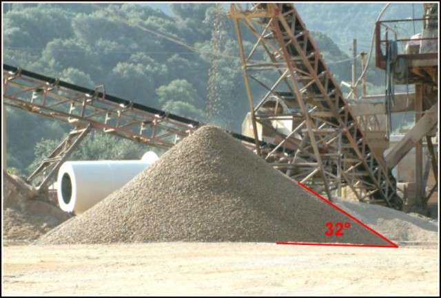
The angle of repose of gravel and crushed stone is from 30 to over 40 degrees depending on the angularity of the grains, whether they are dry or we. Here 32 degrees is shown. 45° can exceptionally be reached in nature or artificially crushed stone beds with very sharp-edged gravel and additional large blocks or fine grains.

Loose gravel and stone heaps form the same angle of repose, regardless of whether they are dry or wet. Sand and even fine gravel, however, must be absolutely dry in order to estimate φ on the basis of θ, as the grains tend to stick to each other given the slightest moisture and thus form a steeper θ than φ which is measured by other methods. Thus the φ of these materials ranges from about 30 to 45 degrees, depending on the angularity and size distribution of the grains. 45 degrees or just above is a high value that is reached only by very sharp-edged material such as of artificially crushed gravel or rubble containing an optimal mixture of large angular blocks and finer grains.

In the case of fine-grained, cohesive soils, this method cannot be applied, because of the angle of repose θ is strongly influenced by the cohesion of the material c and says little about the angle of friction φ. In these soils φ must be measured with special laboratory methods and is generally smaller than 30 degrees.

Such a lab method used the so-called triaxial device. https://en.wikipedia.org/wiki/Triaxial_shear_test It is called such because the sample is loaded along all three main axes of the rectangular coordinate system. For most devices, the forces along two of the axes are the same and the experiment can be evaluated quasi-two-dimensionally. A cylindrical soil sample is placed in a transparent pressure-proof container and is loaded using hydrostatic pressure usually with water. A rubber membrane around the sample prevents the sample absorbing water. A pair of dies along the longitudinal axis of the cylinder allow exerting additional pressure on the end surfaces. Thus the conditions are created to load the soil sample for example as if at at a certain depth, and with additional defined stresss.

In order to measure the shearing parameters φ an c using a triaxial device, the hydrostatic pressure of the device is brought to a desired value, and then the pressure on the end surfaces is increased until the sample develops fracture surfaces (faults). Unlike in a shear box, the exact location of a fault surface is not known beforehand. Depending on the material, it is a single surface at a well recognizable angle, or there are multiple parallel or even intersecting fracture surfaces. The angle already shows φ, because to the longitudinal axis it is 45° - φ/2, or to the end face 45° + φ/2. However φ is not determined in this way, but rather from a diagramm drawn using measurements from several tests with different stress values. Then both both φ and any cohesion c can be determined. It may show that φ is not a constant, but varies somewhat according to stress.

There are also triaxial devices which work not only statically, but also dynamically, e.g. for simulating the conditions from earthquakes.

There are different variants of the shearing parameters. It depends on whether the sample is consolidated before the measurement, and whether drained or not. A sample of the soil tested as described above gives non-consolidated, undrained values. If however the end surfaces are are porous and let pore water escape during compaction, then drained values are given. Alternatively the pore pressure can be measured instead of drining. Which of the variants are needed, depends on the situation, e.g. belonging to a defined measurement procedure.

Instead of with forces, we can define φ with stresses, as will be described further below. φ is the arc tangent of the normal stress divided by the shear stress. If soil is loaded non-uniformly, for example, by a surcharge or a wall, stresses and forces with different directions are produced. Below a certain threshold, the soil is able to endure this without moving. This corresponds to the static friction e.g. between two stones, as described above. Above this threshold, fractures and fault surfaces appear; one part of the soil is moved against another part.

Properties of sand

Sand has properties of both coarser and finer soils. Dry sand trickles through your fingers. Damp sand, however, although not cohesive, has an apparent cohesion (max. 8 kN/m²) and can be shaped. Every builder of sand castles makes use of this!

Advanced properties of sand: The slope angle θ of dry sand is roughly 30 degrees. If the sand is compacted, both θ as well as friction angle φ become greater, but φ more than θ. Ghazavi et al. (2008) give a relationship: θ = φ/3 + 22°. For example, if θ and φ of a sample of loose sand are initially both 33°, when compacted θ can reach 35°, yet φ can become 39°.
Schwing (1991) gives a relationship between φ and density ρ for a certain standard sand: For φ between 37° and 43°, the following applies: φ = 62,5° ∙ (ρ - 1). Here ρ is entered in units of tonnes/m³ but the unit not evaluated. According to this formula, loose sand with ρ = 1.35 t/m³ would have a φ of approx. 22°. If it is compacted to ρ = 1.5 t/m, φ grows to approx. 31°. The two formulas do not match completely because they apply only to those sands with which they were created. They serve here to illustrate the relationships.

The properties of sand change strongly depending on the water content. The slope angle θ increases with increasing water content and can be perpendicular or overhanging around roughly 20% water content. At 25% or more, θ becomes rapidly smaller. In the case of saturation, and after movement θ reaches a minimum of about 12°. Completely under water, however, θ increases to 20-30°. Upwards percolating water and/or movements can cause sand to liquefy, then one speaks of quicksand. Here θ is very small and also the load carrying capacity decreases drastically. Therefore the water sensitivity must be considered at all times when constructing dry stone walls in sandy environments.

Properties of fine-grained soils

The properties (consistency, c, φ, γ) of cohesive fine-grained soils vary depending on their composition and water content. Loams may swell with water uptake and shrink when dry, often making cracks. For dry stone construction it is mainly important to know whether a loamy soil is mainly sandy, silty or clayey. Sandy soils have larger pores and drain well. Clayey soils hold water and are pretty impermeable. But when they are dry, clayey soils are even suitable as building materials, e.g. in the form of clay bricks. Their grains are often small platelets which bind particularly tightly to each other. Aqueous clay is slippery because the platelets form layers which slide easily. Silty soils are the least stable and most sensitive to frost.

When wet soil freezes it is then temporarily firm. Upon thawing, it loses part of its load-bearing capacity. If during the freezing additional water (e.g., the melt water from a puddle) is present and the soil is silty, this can cause frost heave due to the formation of ice lenses (see Faber 1932).

Soil improvement

Base layer

Mature (grown) soils are usually firm enough as a base for dry stone walls. Even cohesive, clayey soils may be viable if they do not get too wet. However if the soil is recognizably soft or prone to water retention, there are several ways to remedy the situation.

• By widening the foundation the pressure on the ground is reduced and is also partially transferred to deeper, generally firmer layers (see image below). If large, flat and uniform foundation stones are available, this also reduces the risk of irregular subsidence and the ground is somewhat protected.

• Another option is to deepen the foundation. As much soil is removed until the sole appears to be sufficiently firm. Instead of just removing the grass or the top 15 centimeters, it can amount to 30 to 50 centimeters. If movements due to frost must be totally avoided, the foundation must extend below the frost line, usually about 80 centimetres in the lower parts of Switzerland and much more in the mountains. A frost-free foundation is however not normally necessary.

• Since such a deep foundation requires a lot of stone, a third option can be more cost-effective: Replacing the soft soil not with foundation stones but instead with a base consisting of a gravel-sand mixture. The supplied material is initially loose with large spaces between the grains. By tamping or vibrating the hollow spaces are reduced by the migration of the finer grains into these. This process can be accelerated with the addition of water. As a result, the new material is compacted. The gravely base-layer is not only firm and frost-resistant, but also well-draining.

The compaction of a soil surface can be easily estimated "by foot". The foot-pressure of a person corresponds approximately to the pressure of a dry stone wall as high as this person. Balancing on one heel or on toes, more than ten times this pressure can be reached. So the bearing suitabilty of the soil surface can assessed even for relatively high walls. However this method says nothing about the deeper layers of the soil. In order to assess these, geotechnical procedures have to be applied, e.g. penetration tests. In the case of developed soils, the bearing capacity tends to increase downwards. At the same time, the vertical pressure decreases with depth (see picture). Therefore, after the removal of the top soil, as soon as the foot test indicates a sufficiently firm surface, the soil underneath can also be expected to to be sufficiently firm.

Vertical soil pressure: A wall with weight G and width b exerts on the ground a vertical pressure of G/b per unit length. The curves on the right show approximately the pressure bulb according to Boussinesq, lines with a constant vertical pressure as a percentage of G/b. The depth at the 20% line and 2.5 b is called the significant depth (see Murthy (2003)). On the left side is shown the simpler 2:1 rule: It is assumed that the pressure is limited by a trapezoid with inclination 2:1 and decreases. Thus, at a depth of b it decreases to 50%, about in line with the pressure bulb. Further down the rule is less accurate. But also the Boussinesq-lines are only a model for a certain ideal soil and would be different for other soils.
The image also shows why a compacting device cannot appreciably compact the soil below the significant depth. Therefore soil to be artificially compacted should be built up and compacted in several thin layers.

Settlement and ground failure

When a wall is freshly built on soil, it will sink in somewhat. Some settlement will always occur except on solid rock. In the case of a firm, non-cohesive soil, the largest part of the settlement occurs immediately due to grain rearrangement and is usually a few millimeters. In the case of cohesive soil, there is usually a settlement of a few centimeters within several days or weeks, but the settling process may continue for months or years, depending on the rate at which pore water is expelled, and reach a considerable magnitude

Uniform settlement is rarely noticed. Because of their flexibility, drystone walls are also not very sensitive to uneven settling. However the wythes of free-standing drystone walls may break apart if the lateral bonding is insufficient, e.g. because of too few tie-stones. The longitudinal bonding could also fail if one wall section settles too much. Recognizably weak soil areas can be relieved or overbridged with arches.

The requirements of retaining walls to the supporting soil and base are particularly high. The earth pressure tries to push the wall to the outside and tilt it. Therefore the area under the toe of the foundation is particularly heavily loaded. With the application of the usual factors of safety against tilting (see XX), the pressure may be approximately 1.5 to 3-fold compared to that of a uniformly loaded foundation.

In the case of the soil being overloaded, a ground failure occurs. The wall sinks in relatively rapidly until the pressure diminishes, e.g. because it tilts. The ground breaks along a curved surface (see image below). Therefore with heavily loaded retaining walls, care must be taken to have a sufficient bearing capacity of the soil, especially under the toe. Sometimes the foundations of retaining walls therefore have a widened base. The maximum pressure possible, multiplied by the chosen factor of safety, must be less than the bearing capacity of the soil. To determine and calculate this accurately is difficult because in addition to the width and depth of the foundation, also several soil properties affect the result. The bearing capacity also decreases if the ground in front of the wall drops directly and/or steeply.

For rough estimates, guidelines with standard values are sufficient to see whether there is a problem at all. However, these values, including the safety factor, are usually only used for temporary or subordinate purposes. The guidelines of the US armed forces (1992), for example, comparable with the British standard BS 8004, give following rounded values:

• Soft loamy soil can be loaded with 50 kN/m² - this corresponds approximately to the foot pressure of a heavy person - and would therefore already be a borderline case for a retaining wall of one meter in height.

• Sands with medium compaction can tolerate about 250 kN/m² and gravel sands about 500 kN/m².

• Well-graded and very dense gravel sands as well as solid clay go up to 1000 kN/m².

• Solid rock can be loaded up to 2000 kN/m² (sediments) and over 7500 kN/m² (crystalline rock).

Therefore, ground failure in dry stone walls is usually not an issue, unless they are particularly high or stand on particularly steep terrain, or the soil is unknown, particularly soft or inhomogeneous, or could become so. In these cases a more exact clarification by a civil engineering office is necessary.

If a ground failure occurs not only locally, but the entire slope, including the retaining wall, slides down, this is referred to as a terrain failure.

Base failure and tilting in a retaining wall. The arrows at R show the forces when a retaining wall designed with a (tilting) safety factor of approx. 3 is loaded until it tilts. According to Dörken&Dehne (2004) and VSS (1966), the curves show approximately the theoretical course of fracture lines of a horizontal soil with friction angle φ - here 30°. If the bearing capacity of the ground is exceeded by the pressure of the wall, it sinks and tilts, with the ground swelling out on the downhill side (drawn in red). Since the earth pressure now decreases, the wall can find a new equilibrium if it is well built; otherwise it fails.

Improvement of the backfill as filter layer

As already described in the "Knowledge" section of this book - and again later in the practical building section - a fresh backfill can be built up to act as a filter. This prevents the wall or the backfill itself from being clogged with fine material, which would increase earth pressure and water pressure. The observance of so-called filter rules guarantees the filter stability of the backfill and thus the permanent permeability and drainage of the wall. These rules refer to the distribution of grain sizes in the backfill in relation to the existing soil. Such calculated filter layers are used mainly in the construction of earth dams and squares. Theoretically, they could also be used for drywall construction. In practice, this happens more by intuition than by calculation:

First, a layer of the largest existing stones of preferably equal size is laid. Then a layer of smaller stones is placed, but not so small that they can fall through the gaps of the previous layer. This is repeated, layer by layer, up to the finest available material.

Filter rules according to Terzaghi: Theoretically an exact procedure is possible: The grain size distribution of the backfill material is determined and sorted by sieving. If the grain distribution lines of the different sieve passages in the grain distribution diagram are approximately parallel, the widely used Terzaghi filter rules can be applied, layer by layer according to these definitions:

In construction standards the filter rules are partly to be found with the value 5 instead of 4.

The application of filter rules requires knowledge of the particle size distribution in soil and filter materials or the targeted mixing of the filter materials. With narrowly stepped, round grains of the ideal size, five layers up to a size of 10 cm are theoretically sufficient for a perfect filter. In practice, horizontal surfaces such as squares are built with fewer but specially composed layers so that they drain well. Although the use of dry stone walls is theoretically conceivable, it is rather unrealistic in practice, except roughly as described above and in the building section of the book.

Soil and Earth Pressure

The cross-section to be provided for a retaining wall depends on the maximum earth pressure to be expected from the soil. This in turn depends on many of the soil properties described above, as well as on the inclination of the terrace above the retaining wall and any loads on it.

Druck oder Spannung?

Die Bezeichnung Erddruck ist erklärungsbedürftig. Eigentlich wäre der Begriff Bodenspannung angebrachter. Einerseits, da in der Geotechnik auch sonst eher von Boden als von Erde die Rede ist, und andererseits, da der physikalische Begriff Druck nur ein Spezialfall der mechanischen Spannung beschreibt, nämlich den Betrag der sogenannten Normalspannung, welche unten erklärt wird. Druck ist ein Skalar, d.h. ein Wert mit einem Betrag, der sich auf einer Skala darstellen lässt, aber keine eigene Richtung hat. Spannung bezeichnet einen Betrag, der in einer bestimmten Richtung wirkt. Eine Spannung kann als Vektor dargestellt werden, z.B. grafisch als Pfeil. Die Länge des Pfeils stellt den Betrag der Spannung dar, und sein Winkel ihre Richtung. Trotzdem hat sich das Wort Erddruck etabliert und wird oft auch dort verwendet, wo eigentlich eine Spannung gemeint ist. (In der Elektrizität ist der Gebrauch der Wörter anders herum: hier bezeichnet die elektrische Spannung eine skalare Grösse!)

Die mechanische Spannung σ (sigma) bezeichnet die Kraft pro Flächeneinheit, die auf eine beliebig geneigte, gedachte Schnittfläche wirkt. Eine Spannung kann aus mehreren speziellen Spannungen zusammengesetzt werden, die als Vektoren addiert werden. Wirkt eine Spannung senkrecht, d.h. normal zur Fläche, heisst sie Normalspannung (σN) und entspricht dem Druck p. Wirkt sie tangential zur Fläche, heisst sie Schubspannung oder Scherspannung τ (tau). Eine ruhende (statische) Flüssigkeit kann keine Reibung und somit keine Scherspannung entwickeln, sondern nur einen hydrostatischen Druck. Eine Flüssigkeit, die in Bewegung ist, entwlckelt jedoch eine hydrodynamische Spannung, welche Reibung, Staudruck und Auftrieb bewirkt, letztere zusätzlich zum allfälligen statischen Auftrieb. Somit ist ein Wehr stärker beansprucht als ein Damm. Flüssigkeiten können auch Oberflächenspannungen haben. Diese sind nur bei kleinen Dimensionen wirksam und bewirken z.B. die Saugwirkung eines Schwamms oder feinkörnigen Bodens.

Nochmals, aber anders herum: Der Druck p bezeichnet die Kraft pro Flächeneinheit, die senkrecht oder normal, d.h. im rechten Winkel, auf eine Fläche wirkt. Der Druck hat keine Richtung, d.h. in jeder Richtung denselben Wert, nämlich den Betrag der Normalspannung σN. Dies ist im Fall des hydrostatischen Drucks einer Flüssigkeit, z.B. Wasserdruck, leicht überprüfbar. Die durch eine Flüssigkeit auf eine Fläche ausgeübte Kraft ist immer gleich, egal ob die Fläche horizontal, vertikal oder schräg angeordnet ist. Sogar nach oben wirkt die Kraft; dies ist der statische Auftrieb, welcher z.B. ermöglicht, dass ein Schiff oder eine Eisschicht auf dem Wasser schwimmt.

Alle Böden besitzen eine innere Reibung und manche auch eine Kohäsion. Dadurch können sie, anders als Flüssigkeiten, bis zu einem gewissen Grad mechanische Spannungen aufnehmen. Die Berechnung beliebiger räumlicher Spannungen ist recht kompliziert, kann jedoch oft quasi-zweidimensional erfolgen. Weitere Vereinfachungen ergeben sich, wenn die Achsen des gewählten Bezugssystems den Richtungen der sogenannten Hauptspannungen entsprechen. Diejenige Spannung mit dem höchsten Betrag wird die erste Hauptspannung σ1 genannt, diejenige mit dem kleinsten Betrag σ3. Im Boden entsprechen meistens σ1 der Normalspannung σN und σ3 der Scherspannung τ.

Vertikaler Erddruck und Ruhedruck

Der einfachste Fall ergibt sich z.B. bei einer Ebene aus kohäsionslosem, körnigen Boden, die nicht durch Auflasten und Wände tangiert wird. Die Hauptspannung σ1 entsteht durch das Gewicht des Bodens und zeigt vertikal nach unten, kann also auch mit σv bezeichnet werden. Die Zunahme gegen unten ist bei homogenem Boden wie bei Wasser praktisch linear. Tatsächlich ist es ein bisschen mehr, da die Verdichtung und somit die Dichte in der Tiefe etwas grösser als nahe bei der Oberfläche sind. In erster Näherung entspricht σv der mittleren Wichte Υ mal der Tiefe an der betreffenden Stelle bzw. der Höhendifferenz zur Oberfläche Δh:

σ_v = Υ ∙ Δh

Bei Wasser wirkt der hydrostatische Druck in alle Richtungen, also ist der seitliche Druck genau gleich stark wie der vertikale und hat denselben Betrag wie σ_v. Bei Boden ist die seitliche, horizontale Spannung σ_h bzw. σ₃ jedoch kleiner, und zwar um den sogenannten Beiwert des Ruhedrucks, k₀. Dieser entspricht etwa (1 – sin φ) und variiert von etwa 0,3 für die grössten vorkommenden Reibungswinkel, bis zu 1 für einen vollkommen verflüssigten Boden.

σ_h = σ_v ∙ K₀ = Υ ∙ Δh ∙ (1 – sin φ)

~0,3 < σ_h < 1

Dieser Ruhedruck wirkt nicht nur im schrankenlosen Gelände, sondern auch als Erddruck auf eine vertikale Wand, wenn diese absolut unbeweglich ist, z.B. auf die massive Kellerwand eines Gebäudes. In der Geotechnik wird dafür das Symbol e0 verwendet.

Die meisten Stützwände und besonders Trockenmauern können jedoch als beweglich angenommen werden. Sie geben dem Erddruck ganz wenig nach, der Boden entspannt sich und dadurch wird der Erddruck kleiner. Bei der kleinsten Bewegung, z.B. Kippen um den Fusspunkt, muss der Boden aktiv nachrutschen, um weiterhin einen Druck ausüben zu können. Dieser Druck heisst aktiver Erddruck e_a und ist wesentlich kleiner als der Ruhedruck e₀. Es ist bei Stützmauern meistens zulässig, mit dem aktiven Erddruck zu rechnen, und er wird unten ausführlich beschrieben.

Passiver Erddruck

Umgekehrt gibt es den passiven Erddruck e_p, der entsteht, wenn eine Fläche gegen den passiven Widerstand des Bodens bewegt wird. Hier muss der Boden nach oben ausweichen und drückt besonders fest gegen die Fläche. Der passive Erddruck ist wesentlich stärker als e_a und e₀, wie man sofort merkt, wenn man z.B. versucht, eine leicht gekippte Stützmauer wieder aufzurichten: Es braucht enorme Kräfte. Eine weitere Verwendung von ep ergibt sich bei einer tief eingegrabenen, monolithischen Mauer. Hier kann e_p des eingrabenen Teils ausgerechnet werden. Dieser bewirkt einen zusätzlichen Widerstand insbesondere gegen das Gleiten. Bei Trockenmauern bringt das wenig. Die meisten Trockenmauern werden nicht sehr tief eingegraben, so dass nur der lockere Oberboden passiven Widerstand leisten kann. Dieser ist schwach und kaum quantifizierbar. Wird die Trockenmauer doch tief eingegraben, werden die unteren Steine zwar nicht gleiten, jedoch dürfte sich bei Überlastung eine Bruch- oder Gleitfläche etwa auf Höhe der talseitigen Erdoberfläche bilden und die Trockenmauer dort gleiten oder kippen. Aus diesen Gründen wird der passive Erddruck hier nicht weiter beschrieben.

Aktiver Erddruck

Der Erddruck e_a auf eine Mauerstelle ist umso größer, je größer die Wichte des Bodens und die Neigung sowie Belastung der Terrasse sind und je kleiner sein innerer Reibungswinkel φ und seine Kohäsion c sind. Die folgenden Ausführungen beziehen sich immer auf ein kurzes Mauerstück innerhalb einer Mauer; die Verhältnisse an den Enden, Ecken, Kurven oder Mauerköpfen werden nicht betrachtet.

1756 hat der bekannte Physiker Coulomb eine Erddruck-Theorie präsentiert, die mit neueren Anpassungen auch heute eingesetzt wird. Die Theorien sind auch heute nicht für alle Böden und Bedingungen exakt gültig, jedoch weitgehend (vgl. Heymann 1997).

Maßgebend für die Berechnung des Erddrucks nach Coulomb ist ein Beiwert der K_a genannt wird. Oft wird die horizontale Komponente davon verwendet, genannt K_ah. Dieser liegt immer zwischen Null und eins und ist abhängig vom Reibungswinkel φ des Bodens, der Terrassenneigung β, dem Anzug der Mauerrückseite α sowie der angenommenen Reibung zwischen dieser und dem Boden. Der dieser Reibung entsprechende Winkel δ wird später beschrieben.

Die Formeln für K_a und K_ah sind:

         und 

K_a und K_ah unterscheiden sich also nur durch den Faktor cos(δ-α). Sie werden auch in geotechnischer Software und normativen Empfehlungen benutzt und – meistens nur K_ah – in Tabellen zugänglich gemacht. Manchmal findet man auch die Bezeichnung K_agh. Mit einem dieser Tabellenwerte lässt sich der Erddruck ohne weitere mathematischen Methoden oder physikalischen Kenntnissen berechnen.

Zunächst besteht der totale aktive Erddruck aus mehreren Komponenten, welche mit einem weiteren Suffix an zweiter Stelle bezeichnet werden. Der gewichtsbezogene Teil (Suffix "g") entsteht durch das Eigengewicht des Bodens. Ein weiterer Teil entsteht durch den Druck P von Auflasten auf der Terrasse (Suffix "p", nicht zu verwechseln mit dem "p" beim passiven Erddruck). Bei bindigem Boden gibt es eine Zugspannung durch die Kohäsion (Suffix "c"), die abgezogen wird. Der gesamte aktive Erddruck ist also:

e_a = e_ag + e_ap - e_ac

Für e_ag gilt eine ähnliche Formel wie beim oben beschriebenen Ruhedruck, nur dass K_a statt K₀ verwendet wird:

e_ag = Υ ∙ Δh ∙ K

Für e_ap ist es noch einfacher, allerdings nur wenn die Terrassenneigung Null ist oder die Rückwand senkrecht ist (sonst siehe weiter unten). Dann produziert eine allfällige Auflast P einen Erddruck:

e_ap = P ∙ K_a

Den meistens nicht verwendeten Term e_ac lassen wir hier mal ausser Acht; weiter unten steht etwas dazu.

Wasserdruck

Wasserdruck (mit φ = 0) rechnet sich genau gleich, aber einfacher, denn der Beiwert Kah ist schlicht 1, bzw. unnötig. Es gibt keine Unterscheidung zwischen aktivem, passivem oder Ruhedruck: sie sind identisch. Es gibt keine Auflasten (sie müssten schwimmen) und keine Kohäsion, somit keine "p" und "c" Komponenten. Der Wasserdruck wirkt immer genau rechtwinklig auf die begrenzende Fläche.

Ein häufige Fehlerquelle ist allerdings die Verwechslung von K_ah und K_a. Bei nicht-senkrechten Wänden ist K_a nicht 1, sondern 1/cosα.

Soll eine Kombination von gleichzeitigem Erddruck und Wasserdruck berechnet werden, muss noch der Auftrieb durch das Wasser berücksichtigt werden. Dies kommt bei sich selber entwässernden Trockenmauern jedoch selten vor.

Silodruck

Erd- und Wasserdruck nehmen von der Mauerkrone oben bis zum Mauerfuß unten zu. Bei Wasserdruck ist die Zunahme fast exakt linear und vollkommen unabhängig von der Form der Mauer oder des Geländes hinter der Mauer: Ein Spalt von einem Millimeter erzeugt exakt denselben statischen Druck wie ein ganzer Ozean. Bei Erddruck bestehen ähnliche Abhängigkeiten, wenn angenommen wird, dass das ganze Material homogen und nicht durch stabiles Gelände oder Felsen eingeengt ist. Existieren aber solche Begrenzungen, nimmt der Erddruck gegen unten weniger stark zu und entspricht dann eher dem sogenannten Silodruck.

Erddruckkraft und Angriffspunkt

Bis hierher war die Rede von Spannung oder Druck. Für weitere Berechnungen wird die Erddruckkraft benötigt, welche entsteht, wenn der Druck auf eine definierte Fläche wirkt.

Aus der Druckverteilung an der inneren Mauerfläche lässt sich für jedes Stückchen Mauerfläche die entsprechende Kraft ausrechnen. Computerprogramme können sich Stückchen für Stückchen numerisch durch die Mauer rechnen. Für die analytische Berechnung von Hand werden die Kräfte – pro Längeneinheit der Mauer – zu einer einzigen Erddruckkraft zusammengefasst, die an einem Punkt in einer Richtung wirksam ist. Eine solche Kraft gibt es nicht wirklich, aber sie lässt sich so berechnen. Dies ist eine schematische Vereinfachung, denn sie lässt sich für Trockenmauern nur anwenden, wenn sich die Mauer beim Gleiten und Kippen zunächst wie ein einziger Körper verhält und der Boden am Drehpunkt nicht nachgibt. Das ist bei vielen Trockenmauern annähernd der Fall.

Betrag

Der Betrag der ganzen gewichtsbezogenen Erddruckkraft Eag errechnet sich – bei homogenem Boden - als Wichte des Bodens mal das Integral des Erddrucks eag über die Stützhöhe.

Das Integral des Drucks über die Mauerhöhe ist bei einer homogenen Schicht einfach der mittlere Druck – also Wichte mal Ka mal halbe Höhe. Daraus ergibt sich die Kraft pro Längeneinheit Mauer, wenn nochmals mit der Höhe multipliziert wird. Als Formel:

Die zweite Kraft Eap durch Auflasten wie die Verkehrslast, rechnet sich am einfachsten durch die Annahme eines gleichmäßigen Drucks P auf der gesamten Terrasse. Dann ist:

Der letzte Teil fällt meistens weg, nämlich wenn α oder β Null sind. Natürlich können auch Punkt- bzw. Linienlasten berechnet werden, oder Terrassen mit unterschiedlichen Winkeln und Belastungen. Auf solche wird im Folgenden nicht eingegangen; es empfiehlt sich die Verwendung einer Erddrucksoftware (vgl. hierXX).

Die Erddruckkraft ist bei bindigen Böden durch deren kohäsionsbedingte Komponente Eac reduziert. Dies kann mit Hilfe von relativ unhandlichen Gleichungen ausgerechnet werden (vgl. Schwing 1991). Einfacher ist die Anwendung von Tabellen mit entsprechenden Beiwerten oder wiederum Software. Überschlagsmäßig kann verwendet werden:

Dies gilt mindestens wenn α und β = 0. Die Kohäsionsspannung c kann bei bindigen, nicht allzu weichen Materialien 5-20 kN/m² betragen, in festeren Zuständen sogar ein Mehrfaches davon. Damit wird die Belastung selbst durch grössere Auflasten negiert, bei niedrigen Mauern sogar die ganze Erddruckkraft aufgehoben. Das heißt, ein stabiler bindiger Boden, dessen senkrechte Böschung von alleine hält, braucht zunächst gar nicht gestützt zu werden. Die Verwendung der Komponente Eac hat aber einen gefährlichen Haken. Da sie als Zugkraft wirkt, kann sie verschwinden, wenn sich im Boden Risse oder Bruchflächen bilden. Und der Wert hängt auch stark von der Menge des eingebundenen Wassers ab. Deshalb sollte nur mit der Kohäsionskraft gerechnet werden, wenn sie zuverlässig bestimmt wurde und sicher ist, dass sie beständig ist. Ein solcher Nachweis kann in der Regel nur von bodenkundigen Fachleuten vorgenommen werden. Außer bei untergeordneten, nicht sicherheitsrelevanten Stützmauern, wird man deshalb oft mit Eac = 0 rechnen müssen, wie auch ohnehin bei nicht-bindigen Böden.

Angriffspunkt

Der wirksame Angriffspunkt der Erddruckkraftkomponente E_ag ist nicht in der Mitte der Mauerrückseite, wie man meinen könnte, sondern bei 1/3 der wirksamen Höhe von unten, wie sich zeigen lässt (siehe auch die folgende Abbildung). Hingegen ist der Angriffspunkt der Komponente E_ap tatsächlich in der Hälfte. Diese Angaben sind wichtig, wenn es um die Berechnung der Kippstabilität der Stützmauer geht. Hierfür müssen E_ag und E_ap als Vektoren summiert werden, während es für die Berechnung der Gleitstabilität genügt deren Beträge zu summieren.

In dieser Abbildung der Erddruckkräfte werden der Übersichtlichkeit wegen nur deren horizontalen Teile gezeigt. Die horizontale Pfeile zeigen die horizontale Komponente des Erddrucks e von oben Null bis unten maximal. Die Erddruckkraft E_agh entspricht dem Integral, also der Fläche des Dreiecks. Dieses ist gleich groß wie das rosa Rechteck. Deren Betrag ist also h mal dem Erddruck bei h/2. Die Kraft wirkt jedoch am Schwerpunkt des Dreiecks. Dieser liegt am Schnittpunkt der Seitenhalbierenden, also bei h/3.
Die Auflast P (vertikale Pfeile einer gleichmässigen Flächenbelastung) erzeugt einen seitlichen Druck P mal K_ah. Dieser ist dem Erddruck überlagert, hier der Übersichtlichkeit wegen nach rechts verschoben. Der Schwerpunkt der rechteckigen Verteilung ist in der Hälfte, somit auch der Angriffspunkt der Auflastkraft E_aph. Die beiden Kräfte können als Vektoren addiert werden, wie hier gezeigt wird.
Die vertikalen Komponenten sind hier nicht dargestellt.

Richtung und graphische Zusammenfassung

Wenn der Boden ganz ohne Reibung gegen die Mauerrückseite drücken würde, würde die Erddruckkraft genau im rechten Winkel zur Fläche wirken, wie das bei Wasser der Fall ist. Tatsächlich drückt die Kraft bei einer Stützmauer mehr von oben, nämlich mit einem Winkel δ (delta) von diesem rechten Winkel aus gemessen. Bei einer perfekten Verzahnung des Bodens mit der Hintermauerung einer Trockenmauer, könnte δ maximal den Reibungswinkel φ des Bodens annehmen. Bei üblichen Stützmauern aus Beton wird δ = 2/3 φ angenommen, bei sehr glatten Wänden ⅓ φ. Bei gut verzahnten Hintermauerungen wie bei den meisten Trockenmauern dürfte δ = 0,9 φ oder δ = φ gelten, aber heutige Trockenmauer-Empfehlungen gehen nach wie vor von δ = 2/3 φ aus, so auch [CAPEB 2007] und [FLL 2012]. Die untenstehende Abbildung von Erddruckkräften ist mit δ = φ gezeichnet. Die Pfeile der Kraftvektoren dieser Abbildung zeigen anschaulich, wie die Erddruckkraft bei verschiedenen Böden und Winkeln der Mauerrückwand aussieht. Immer ohne Verkehrslast und bei einer angenommen Bodenwichte von 18 kN/m³. Die kleinsten Werte ergeben sich bei φ=45° und α=20°: nur 1,1 kN. Die grössten Werte – hier über 16 kN bei α=-20° – entsprechen etwa Treibsand oder "Superschlamm", welches eine aussergewöhnliche, extreme Belastung darstellen würde, denn übliche Schlämme sind entweder weniger schwer oder weniger flüssig. Zum Vergleich auch reines Wasser (γ = 10 kN/m³). In der Praxis stellt Wasserdruck fast immer die größte vorkommende Belastung dar; nur die hochplastischen oder flüssigen Schlämme üben mehr Druck aus. Bei der Terrassenneigung β = 20° sind keine niedrigen φ-Werte möglich, sie sind deshalb nicht angegeben. Zwischen den φ-Werten kann interpoliert werden; dazu dienen die gezeichneten Kurven.

Die gewählte Mauerhöhe in der folgenden Abbildung entspricht (in Meter) der Quadratwurzel von zwei; somit bedeutet die Vektorlänge den Betrag (in kN pro Meter Mauerlänge) der gewählten Bodenwichte von 18 kN/m³ × K_a. Für andere Mauerhöhen h müssen die Werte mit ½ h² multipliziert werden.

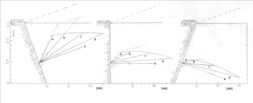
Betrag und Richtung der gewichtsbezogenen aktiven Erddruckkraft E_ag nach Coulomb, in Kilonewton pro Meter Mauerlänge, bei Mauerhöhe h = 1.414 m, Wichte Boden = 18 kN/m³, Terrassenneigung β = 0° und 20°.
Die Kraftvektoren a,b,c,d,und e sind für φ- bzw. δ-Werte von 45°, 30°, 15°, und 5°, sowie 0° (Wasser).

Wasser, Klima und Wetter

Siehe Buch Seite 211

Rechtliche Anforderungen und Besitzverhältnisse

Siehe Buch Seite 212